Change of Variables in Multiple Integrals 

We have already seen that for functions of one variable the chain rule 

at once gives the rule for change of a variable in a definite integral 

There is a formula analogous to this for double and triple integrals. 

Change of Variables for Double Integrals 

Let be a continuous function on a region in the -plane, and let the transformation maps the region in the -plane into the region . Then 

where is the Jacobian and represents either or  

Change of Variables for Double Integrals 

The change of variables formula for triple integrals is similar to the one given above for double integrals. 

Change of Variables for Triple Integrals 

Let be a continuous function on a region in the -space, and let the transformation maps the region in the -space into the region . Then 

where is the Jacobian and the region i -space. 

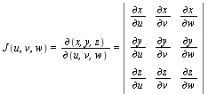
Change of Variables for Double Integrals 

If or is a one-to-one transformation, then or it can be shown that 

1,  1 

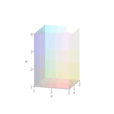
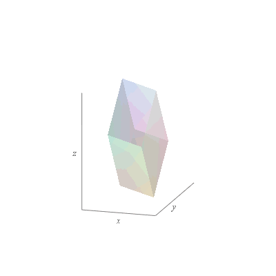
The following commands in the calcplot package plot images of regions under arbitrary coordinate transformations. With these commands we can check whether the description of a new region under a change of coordinates is correct. 

• regionplot2d () plots the image of a region in the -plane of the form , under a coordinate transformation into -plane given by the list  . The variable order is the same as if the int procedure were invoked for a double integral over the region

• regionplot3d () plots the image of a three-dimensional region in -space of the type , , , under a coordinate transformation into -space given by the list . The variable order is the same as if the int procedure were invoked for a triple integral over the region.

In the linalg package
 

• jacobian ( x ..., u,v,...) computes the Jacobian matrix of the vector or list with respect to , v, ...

• det (jacobian)( x(, ...,u,v,...) computes the determinant of the Jacobian matrix

• Jacobian (x(, ...,u,v,...,'determinant') computes the Jacobian matrix and the determinant

Example 1 

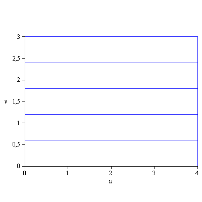
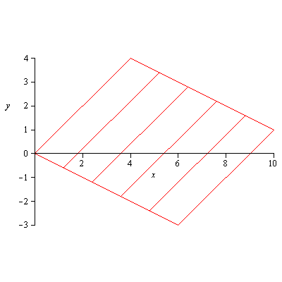
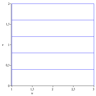
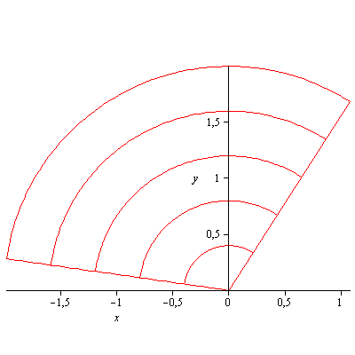
Find the region in the -plane corresponding to the region in the -plane where 

a)   and under the change of variables , .
b) and under the change of variables , . 

Find the region in the -plane corresponding to the region in the -plane where 

c)  , , and under the change of variables , . 

>	restart: MathMaple:-ini():

 

Solution 

a) 

,     > regionplot2d(u=0..4,v=0..3,[u,v],labels=[u,v],color=blue,tickmarks=[6,6]);

,   > regionplot2d(u=0..4,v=0..3,[u+2*v,u-v],labels=[x,y],color=red,tickmarks=[6,6]);

b) 

,   > regionplot2d(u=1..3,v=0..2,[u,v],labels=[u,v],color=blue,tickmarks=[6,6]);

,   > regionplot2d(u=1..3,v=0..2,[v*cos(u),v*sin(u)],labels=[x,y],color=red,tickmarks=[6,6]);

c) 

, ,   > regionplot3d(u=1..3,v=0..2,w=1..4,[u,v,w],style=patchnogrid, lightmodel=light4,labels=[u,v,w],axes=frame,tickmarks=[4,4,4],orientation=[-73,75],transparency=0.5);

,   > regionplot3d(u=1..3,v=0..2,w=1..4,[u+v+w,2*u-v-2*w,-u+3*v-w],style=patchnogrid, lightmodel=light2,labels=[x,y,z],axes=frame,tickmarks=[0,0,0],orientation=[-73,75],transparency=0.5);